
The previous post was dealt with likelihood . Let’s take a look at some interesting examples introduced in “Major League Baseball statistics”. (Book in Korean)
The R markdown can be found in Github and this post is quoted partially from chapter 4 in the book mentioned above.
1. The probability that goes on the base twice in five at-bats given a on-base percentage.

Joey Votto has fabulous on-base percentage at 2015′ and 2016′ season. At that time he got along with Mr.Choo Shin Soo so that he was also well-known in Korea. It is expected that he will be success going on base with 46%. Usually he would get 5 times at batting as a 2nd or 3rd at batting order. Then, what is the probability that he might go on base twice at a game?
First of all, I would really explain the on-base percentage (abbr. OBP) for whom doesn’t know the meaning of it.
The On-Base Percentage is,
It is a percentage how much a hitter can go on-base. It’s said as On-Base Percentage and its abbreviation is OBP. Usually the first hitter in a team may need the high OBP. It can release a tension for the next hitter as well as affect the opponent to feel somewhat pressure.
[Deriving Equation] (Hit + Dead Ball + Base-On-Balls)÷(At bat + Dead Ball + Base-On-Balls + Sacrificed Fly). The on-base count is divided by total attempts at batting position. It is included that on-base from hits, of course, as well as dead balls, base-on-balls. It is rounded from 4th decimal place so as to represent it to 3rd decimal place.
OBP is the probability can be defined in the ratio of success going on-base to the total attempts at-bats. When we say a probability, we should deal with its probability distribution.
If you have some knowledge in statistics, you can assume the OBP (On-Base Percentage) followed as binomial probability distribution with p as success probability. So many trials are independent each other and the probability of success will be p and the one that fails is 1-p.
If we assume k successes and n-k fails, we can derive the binomial probability distribution function such like this.
Pr(k;n,p) = Pr(X=k) =\binom{n}{k} p^{k}(1-p)^{n-k} \cdots (*)
for k = 0, 1, 2,\cdots,n
where \binom{n}{k} = \dfrac{n!}{k!(n-k)!}
Joey Votto is 2nd in batting order so that he used to be 5 opportunities at-bats at a game. Considering his OBP, it is highly expected that he would be going on-base at twice. In the other hand, it’s very rare chance that he would not be on-base or success on-base at all times. If you can think of that, you seem to describe the binomial distribution in your mind.
If we plug-in n=5, k=2, p=0.460 at above equation (*)
^5C_2 \times {0.460}^2 \times {0.540}^3 = 33.32 % is calculated.
On the behalf of direct calculations, we can make a simulation with random seeds with OBP.
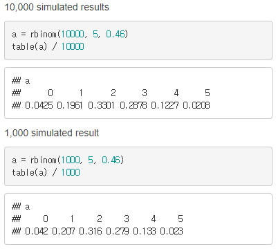
We found that it is almost the same result we have derived from the equation (*).
2. Maximum Likelihood Estimation; To find the OBP which maximizes the probability of going on twice in five at-bats
While we found the probability of going on twice in five at-bats given Joey Votto’s OBP in the previous, now we want to find the most plausible parameter in population when it is observed that going on twice in five at-bats.
If Joey Votto’s On-base percentage is not known and if you watched his next two appearances in five at-bats, even if you’ve been tracking down the on-base percentage needed to maximize the probability that you’ll be able to hit twice on five at-bats in the future, 0.4 is the likelihood that maximizes probability of going twice in five at-bats.
The biggest difference from the probability is that the probability is that you know the on-base percentage, which is the condition of an event (two outs in five at-bats), so you can notice the frequency of two occasions in five. But if you do not know the number of on-base percentage, you have to find the conditions that make the most frequent outbreaks out of five times. That is the likelihood.
From now on, substitute the total number of trials 5 and 2 into the binomial probability distribution function to find the on-base percentage parameter that most improves the likelihood of going out twice in five at-bats.
※ Let’s say “going on twice” as TWICE
P(TWICE)= \binom{5}{2} \times {OBP}^2 \times (1-OBP)^3
(OBP = On Base Percentage)
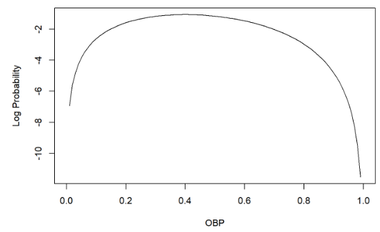
In the maximum likelihood estimation, we can use the characteristic which logarithm increased monotonically. The logarithm of the probability equation is used to find the point at which the slope is zero (that is, the point where the value once differentiated is zero) as the maximum likelihood point.
ln(P(TWICE))=ln( \binom{5}{2} \times OBP^2 \times (1-OBP)^3
= ln10 + 2lnOBP + 3ln(1-OBP)
If we differentiate the equation by OBP,
\dfrac{\partial ln(P(TWICE))}{\partial OBP} = \dfrac{2}{OBP} - \dfrac{3}{1-OBP} = 0
The above formula summarizes OBP = \dfrac{2}{5} =0.4
We obtained the mathematical value that I thought intuitively.
3. Six going on-base cases from five at-bats corresponding a OBP
If a player comes five at-bats, going on-base can be 0, 1, 2, 3, 4, 5 ( six cases)
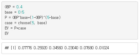
The player with a OBP of 0.4 will be the highest, with 34.56% of the probability going twice in five at-bats. (Following binomial distribution)
It is calculated for six cases in below,
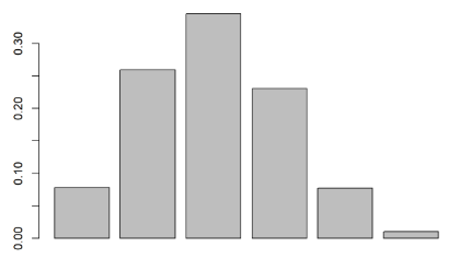
After displaying it with a bar graph, the third bar (when going twice) is the highest, with a slightly tilted distribution to the right.
There are only two reasons for determining the shape of a distribution in a binomial distribution. The Player’s OBP and total trials determine the shape of probability distribution and the probability distribution shape of the players with on-base percentage of 0.3, 0.2 and 0.4 are different.
Let’s compare the shape of probability distributions with on-base percentage of 0.2, 0.3, 0.4, 0.5.
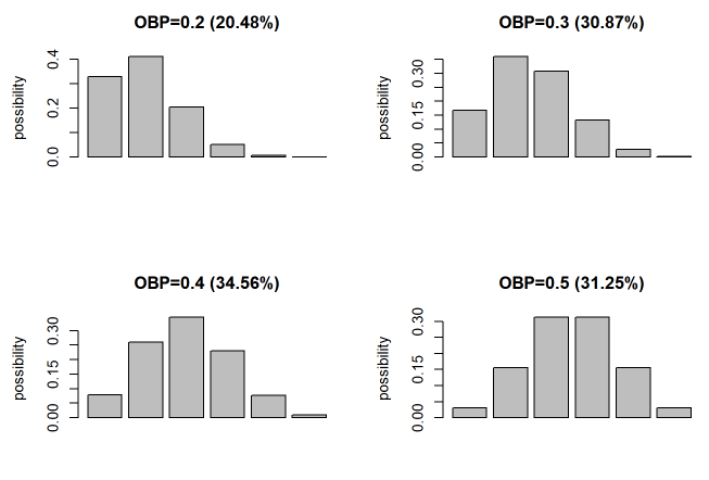
The probability of a 0.2 on-base percentage player being able to go twice in five at-bats is 20.48% and 0.3 on-base percentage is 30.87% and 0.4 on-base percentage is 31.25%.
4. If a player runs 100 games and we observed the each game’s going on-base counts, how we can get the maximum likelihood estimation of parameters ?
I just wondered what would happen if I did not observe only once when a player entered at-bat. He may be able to go on twice on-base in five at-bats similar to the real thing, or he may get on-base once, or he may get on-base all five lucky days.
If we assume P_{OBP} as a player’s OBP which is a parameter of our population, the likelihood can be written by
L(P_{OBP}|x_1,x_2,\cdots,x_n)= L(P_{OBP}|x_1) \times L(P_{OBP}|x_2) \times \cdots \times L(P_{OBP}|x_n)
- i times on-base in five at-bats can be k_i
- Each i on-base can be counted such as n_i . then n_0 + n_1 + n_2 + n_3 + n_4 + n_5 = 100
If we reflect the number of counts of the six on-base cases through 100 observations (competitions), the likelihood function can be obtained as follows.
L(P_{OBP}|x_1,x_2,\cdots,x_n) = {\binom{5}{k_0}}^{n_0} {P_{OBP}}^{k_0n_0} (1-P_{OBP})^{(5-k_0)n_0}\times{\binom{5}{k_2}}^{n_2} {P_{OBP}}^{k_2n_2} (1-P_{OBP})^{(5-k_2)n_2}
\cdots \times{\binom{5}{k_5}}^{n_5} {P_{OBP}}^{k_5n_5} (1-P_{OBP})^{(5-k_5)n_5}
If you take logs on both sides and organize them,
ln(L(P_{OBP}|x_1,x_2,\cdots,x_n)) = n_0ln{\binom{5}{k_0}} + k_0n_0ln(P_{OBP}) + (5-k_0)n_0ln(1-P_{OBP})+ n_2ln{\binom{5}{k_2}} + k_2n_2ln(P_{OBP}) + (5-k_2)n_2ln(1-P_{OBP})
\cdots + n_5ln{\binom{5}{k_5}} + k_5n_5ln(P_{OBP}) + (5-k_5)n_5ln(1-P_{OBP})
If you take derivative by P_{OBP} and set it to 0 and organize it,
0 =\dfrac {\displaystyle\sum_{i=0}^{5} {k_in_i}}{P_{OBP}} - \dfrac {\displaystyle\sum_{i=0}^{5} {(5-k_i)n_i}}{1-P_{OBP}}
\Longrightarrow(1-P_{OBP}){\displaystyle\sum_{i=0}^{5} {k_in_i}} = {P_{OBP}}{\displaystyle\sum_{i=0}^{5} {(5-k_i)n_i}}
\therefore P_{OBP} =\dfrac {\displaystyle\sum_{i=0}^{5} {k_in_i}}{\displaystyle\sum_{i=0}^{5} {k_in_i} + \displaystyle\sum_{i=0}^{5} {(5-k_i)n_i}}
Based on the above equation, I have got n_0, n_1, n_2, n_3, n_4, n_5 values by simulating with some situations such as 1) normal player, 2) good player, 3) bad player.
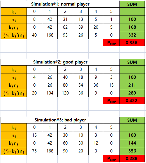
Assuming the binomial probability distribution function with P(OBP) and the number of times on-base(k) according to the number of at-bats (n) as parameters, I could estimate the OBP which is parameter of population by changing the observation counts at 100 games from the method of maximum likelihood estimation.