2.1 What Is Statistical Learning?
X : input variables; predictors; independent variables
Y : output variables; response; dependent variable
Suppose that we observe a quantitative response Y and p different predictors, X_1,X_2,...,X_p . We assume that there is some relationship between Y and X=(X_1, X_2,...,X_p)
《Very general form》
Y=f(X)+\epsilon
2.1.1 Why Estimate f ?
① Prediction
We can predict Y, \hat{Y}=\hat{f}(X)
The accuracy of \hat{Y} as a prediction for Y depends on
1> reducible error
2> irreducible error
E(Y- \hat{Y})^2 = E[f(X) + \epsilon -\hat{f}(X)]^2=\underbrace{[f(X)- \hat{f}(X)]^2}_{\text{reducible}} +\underbrace{Var(\epsilon)}_{\text{irreducible}}
② Inference
We are often interested in understanding the way that Y is affected as X_1,X_2,...,X_p change. In this situation we wish to estimate f, but our goal is not necessarily to make predictions for Y. We instead want to understand the relationship between X and Y. We instead want to understand the relationship between X and Y, or more specifically, to understand how Y changes as a function of X_1,X_2,...,X_p . Now \hat{f} cannot be treated as a black box, because we need to know its exact form. one may be interested in answering the following questions.
Which predictors are associated with the response ?
What is the relationship between the response and each predictor?
Can the relationship between Y and each predictor be adequately summarized using a linear equation, or is the relationship more complicated?
③ Examples
1> Prediction : “Direct-marketing campaign”
Goal : Identify individuals who will respond positively to a mailing
X = demographic variables
Y = marketing campaign (either positive or negative)
2> Inference : “Advertising”
Goal : Answering questions such as :
– Which media contribute to sales?
– Which media generate the biggest boost in sales?
– How much increase in sales is associated with a given increase in TV advertising?
X = advertising media
Y = sales
3> Both prediction and inference : “Real Estate”
Goal :
– How the individual input variables affect the prices?
– Predicting the value of a home given its characteristics.
X = crime rate, zoning, distance from a river, air quality, schools, income level of community, size of houses, and so forth
Y = price of house
2.1.2 How do we estimate f?
① Parametric methods
First step : We make an assumption about the functional form, or shape, of f. For example one very simple assumption is that f is linear in X:
f(x) = \beta_0 + \beta_1X_1 + \beta_2X_2 + \cdots + \beta_pX_pSecond step : After a model has been selected, we need a procedure that uses the training data to fit or train the model.
② Non-parametric methods
Do not make explicit assumptions about the functional form of f. Instead they seek an estimate of f that gets as close to the data points as possible without being too rough or wiggly.
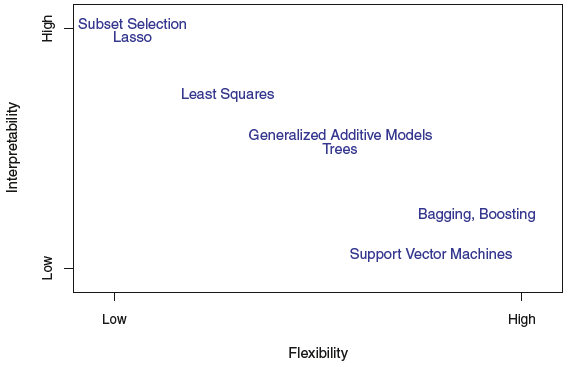
2.1.3 The Trade-Off Between Prediction Accuracy and Model Interpretability
To increase Prediction Accuracy \implies Use more Flexible Model
To increase Interpretability \implies Use Inflexible and Restrictive Model
2.1.4 Supervised Versus Unsupervised Learning
① Supervised : For each observations, there is an associated response measurement
methods : linear regression, logistic regression, GAM, boosting, support vector machines
※ Vast majorities of this book is devoted to this setting
② Unsupervised : We observe a vector of measurements, but no associated response
methods : cluster analysis
③ Semi-Supervised
2.1.5 Regression Versus Classification
Variables can be characterized as either quantitative or qualitative (also known as categorical). Quantitative variables take on numerical values. Examples include a person’s age, height, or income, the value of a house, and the price of a stock. In contrast, qualitative variables take on values in one of K different classes, or categories. Examples of qualitative variables include a person’s gender, the brand of product purchased, whether a person defaults on a debt, or a cancer diagnosis. We tend to refer to problems with
a qualitative response \implies regression problems
a qualitative response \implies classification problems
2.2 Assessing Model Accuracy
2.2.1 Measuring Quality of Fit
In regression setting, the most commonly-used measure is the mean squared error (MES), given by
MES = \dfrac{1}{n}\displaystyle\sum_{i=1}^n (y_i-\hat{f}(x_i))^2
We are interested in the accuracy of the predictions that we obtain when we apply our method to previously unseen test data.
We could compute the average squared prediction error for these test observations (x_0, y_0) .
Ave(\hat{f}(x_0) -y_0)^2In practice, one can usually compute the training MSE with relative ease, but estimating test MES is considerably more difficult because usually no test data are available.
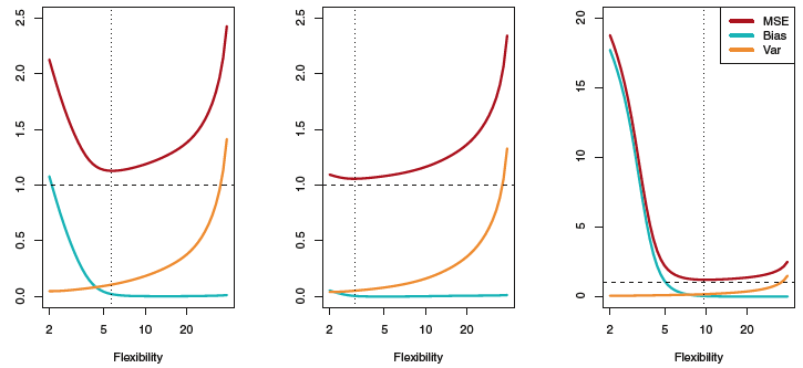
2.2.2 The Bias-Variance Trade-Off
The expected test MSE, for a given value x_0 , can always be decomposed into the sum of the three fundamental quantities: the variance of \hat{f}(x_0) , the squared bias of \hat{f}(x_0) and the variance of the error terms \epsilon . That is,
E(y_0-\hat{f}(x_0))^2 = Var(\hat{f}(x_0)) + [Bias(\hat{f}(x_0))]^2 + Var(\epsilon)
In order to minimize the expected test error, we need to select a statistical learning method that simultaneously achieves low variance and low bias.
What do we mean by the variance and bias of a statistical learning method?
Variance refers to the amount by which \hat{f} would change if we estimated it using a different training data set. Since the training data are used to fit the statistical learning method, different training sets will result in a different \hat{f} . But ideally the estimate for f should not vary too much between training sets. However, if a method has high variance then small changes in the training data can result in large changes in \hat{f} . In general, more flexible statistical methods have higher variance.
On the other hand, bias refers to the error that is introduced by approximating a real-life problem, which may be extremely complicated, by a much simpler model.
As a general rule, as we use more flexible methods, the variance will increase and the bias will decrease.
2.2.3 The Classification Setting
The fraction of incorrect classifications : \dfrac{1}{n}\displaystyle\sum_{i=1}^n I(y_i \neq \hat{y_i})
The test error rate associated with a set of test observations of the form (x_0, y_0) is given by Ave(I(y_0 \neq \hat{y_0})) -(*)
① The Bayes Classifier
It is possible to show that the test error rate given in (*) is minimized, on average, by a very simple classifier that assigns each observation to the most likely class, given its predictor values. In other words, we should simply assign a test observation with predictor vector x_0 to the class j for which
The Bayes classifier produces the lowest possible test error rate, called the Bayes error rate. The error rate at X=x_0 will be 1-max_jPr(Y=j|X=x_0)
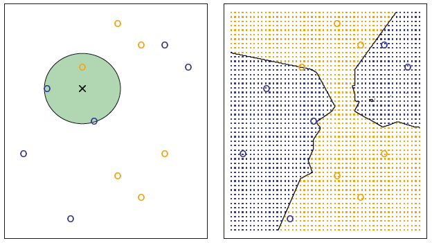
② K-Nearest Neighbors
In theory we would always like to predict qualitative responses using the Bayes classifier. But for real data, we do not know the conditional distribution of Y given X, and so computing the Bayes classifier is impossible. Therefore, the Bayes classifier serves as an unattainable gold standard against which to compare other methods. Many approaches attempt to estimate the conditional distribution of Y given X, and then classify a given observation to the class with highest estimated probability. One such method is the K-nearest neighbors (KNN) classifier. Given a positive integer K and a test observation x_0 , the KNN classifier first identifies the K points in the training data that are closest to x_0 , represented by N_0 . It then estimates the conditional probability for class j as the fraction of points in N_0 whose response values equal j :